Scientific Article LaTeX Template
A free LaTeX scientific article template with the standard article class: title, abstract, sections and references laid out, so you can concentrate on the content.
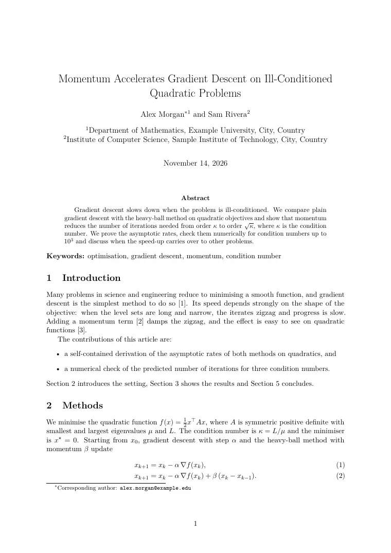
LaTeX source
% Scientific article template: title, authors with affiliations, abstract and keywords, numbered sections,
% theorem, table, plot and bibliography. It is filled with a short example (momentum on quadratic problems)
% so you can see how each part works. Replace the text, the table and the plot with your own.
\documentclass[a4paper,11pt]{article}

\usepackage[T1]{fontenc}
\usepackage{lmodern}
\usepackage[english]{babel}
\usepackage[margin=2.5cm]{geometry}
\usepackage{microtype}
\usepackage{amsmath,amssymb,amsthm}
\usepackage{booktabs}
\usepackage{graphicx}  % only needed if you include image files with \includegraphics
\usepackage{authblk}
\usepackage{pgfplots}
\usetikzlibrary{babel}
\usepackage[hidelinks]{hyperref}
% Bibliography: entries live in references.bib; cite them with \cite{key} or \citet{key}
\usepackage[numbers,sort&compress]{natbib}

\pgfplotsset{compat=1.18}
\newtheorem{theorem}{Theorem}
\theoremstyle{remark}
\newtheorem*{remark}{Remark}

% ---- Title and authors: edit these ----
\title{Momentum Accelerates Gradient Descent on Ill-Conditioned Quadratic Problems}
\author[1]{Alex Morgan\thanks{Corresponding author: \texttt{alex.morgan@example.edu}}}
\author[2]{Sam Rivera}
\affil[1]{Department of Mathematics, Example University, City, Country}
\affil[2]{Institute of Computer Science, Sample Institute of Technology, City, Country}
\date{\today}

\begin{document}

\maketitle

\begin{abstract}
  % Summarise the problem, the method, the main result and why it matters, in about 150 words.
  Gradient descent slows down when the problem is ill-conditioned. We compare plain gradient descent with
  the heavy-ball method on quadratic objectives and show that momentum reduces the number of iterations
  needed from order $\kappa$ to order $\sqrt{\kappa}$, where $\kappa$ is the condition number. We prove
  the asymptotic rates, check them numerically for condition numbers up to $10^3$ and discuss when the
  speed-up carries over to other problems.
\end{abstract}

\noindent\textbf{Keywords:} optimisation, gradient descent, momentum, condition number

\section{Introduction}
% Present the problem, what is known, the gap and your contribution.
Many problems in science and engineering reduce to minimising a smooth function, and gradient descent is the
simplest method to do so \citep{boyd2004}. Its speed depends strongly on the shape of the objective: when
the level sets are long and narrow, the iterates zigzag and progress is slow. Adding a momentum term
\citep{polyak1964} damps the zigzag, and the effect is easy to see on quadratic functions \citep{goh2017}.

The contributions of this article are:
\begin{itemize}
  \item a self-contained derivation of the asymptotic rates of both methods on quadratics, and
  \item a numerical check of the predicted number of iterations for three condition numbers.
\end{itemize}
Section~\ref{sec:method} introduces the setting, Section~\ref{sec:results} shows the results and
Section~\ref{sec:conclusions} concludes.

\section{Methods}\label{sec:method}
% Describe the model, the algorithms and the assumptions needed to repeat your work.
We minimise the quadratic function $f(x) = \tfrac12 x^{\top}Ax$, where $A$ is symmetric positive definite
with smallest and largest eigenvalues $\mu$ and $L$. The condition number is $\kappa = L/\mu$ and the
minimiser is $x^{\star}=0$. Starting from $x_0$, gradient descent with step $\alpha$ and the heavy-ball
method with momentum $\beta$ update
\begin{align}
  x_{k+1} &= x_k - \alpha\,\nabla f(x_k), \label{eq:gd}\\
  x_{k+1} &= x_k - \alpha\,\nabla f(x_k) + \beta\,(x_k - x_{k-1}). \label{eq:hb}
\end{align}

\begin{theorem}\label{thm:rates}
  With $\alpha = 2/(L+\mu)$, method \eqref{eq:gd} satisfies $\|x_k\| \le \rho_{\mathrm{GD}}^{\,k}\|x_0\|$ with
  $\rho_{\mathrm{GD}} = \dfrac{\kappa-1}{\kappa+1}$. With $\alpha = 4/(\sqrt{L}+\sqrt{\mu})^2$ and
  $\beta = \bigl(\tfrac{\sqrt\kappa-1}{\sqrt\kappa+1}\bigr)^2$, method \eqref{eq:hb} converges at the
  asymptotic rate $\rho_{\mathrm{HB}} = \dfrac{\sqrt\kappa-1}{\sqrt\kappa+1}$.
\end{theorem}

\begin{proof}
  Diagonalise $A$ and treat each eigenvalue $\lambda\in[\mu,L]$ separately. For gradient descent the
  iterate along that direction is multiplied by $1-\alpha\lambda$, whose modulus is largest at
  $\lambda=\mu$ and $\lambda=L$ and equals $\rho_{\mathrm{GD}}$ for the stated step. For the heavy-ball
  method the pair $(x_k, x_{k-1})$ evolves with a $2\times2$ matrix whose eigenvalues are the roots of
  $z^2-(1+\beta-\alpha\lambda)z+\beta=0$. For the stated $\alpha$ and $\beta$ these roots are complex
  with modulus $\sqrt\beta=\rho_{\mathrm{HB}}$ for every $\lambda\in[\mu,L]$ \citep{polyak1964}.
\end{proof}

\begin{remark}
  Since $-\ln\rho \approx 2/\kappa$ for gradient descent and $\approx 2/\sqrt\kappa$ for the heavy ball, reaching
  a tolerance $\varepsilon$ takes about $\tfrac{\kappa}{2}\ln(1/\varepsilon)$ and
  $\tfrac{\sqrt\kappa}{2}\ln(1/\varepsilon)$ iterations, respectively \citep{nesterov2004}.
\end{remark}

\section{Results}\label{sec:results}
% Present the results without interpreting them; refer to every table and figure in the text.
Table~\ref{tab:iterations} lists the iterations needed to reduce the error by a factor of $10^{6}$, computed
from the rates in Theorem~\ref{thm:rates}, and Figure~\ref{fig:convergence} shows the error bound for
$\kappa=100$.

\begin{table}[htbp]
  \centering
  \caption{Iterations needed to reduce the error by a factor of $10^{6}$.}
  \label{tab:iterations}
  \begin{tabular}{rrrr}
    \toprule
    $\kappa$ & Gradient descent & Heavy ball & Ratio \\
    \midrule
    10   & 69   & 22  & 3.1 \\
    100  & 691  & 69  & 10.0 \\
    1000 & 6908 & 219 & 31.5 \\
    \bottomrule
  \end{tabular}
\end{table}

\begin{figure}[htbp]
  \centering
  % The plot is drawn with pgfplots, so no image file is needed. To use an image instead:
  % \includegraphics[width=0.8\linewidth]{figure.png}
  \begin{tikzpicture}
    \begin{axis}[
      width=0.8\linewidth, height=6cm,
      xlabel={Iteration $k$}, ylabel={Error bound $\rho^{k}$},
      ymode=log, xmin=0, xmax=300, ymin=1e-7, ymax=1,
      grid=major, legend pos=south west,
    ]
      \addplot[thick, domain=0:300, samples=2] {0.9802^x};
      \addplot[thick, dashed, domain=0:300, samples=2] {0.8182^x};
      \legend{Gradient descent, Heavy ball}
    \end{axis}
  \end{tikzpicture}
  \caption{Bound on the error after $k$ iterations for $\kappa=100$.}
  \label{fig:convergence}
\end{figure}

\section{Discussion}
The number of iterations grows linearly with $\kappa$ for gradient descent and with $\sqrt\kappa$ for the heavy
ball, so the advantage of momentum widens as the problem becomes harder: a factor of 3 for
$\kappa=10$ and more than 30 for $\kappa=10^{3}$. The analysis holds for quadratics only; for general
convex functions the heavy-ball method needs other parameters and can fail to converge, which is why
accelerated variants are preferred in practice \citep{nesterov2004}.

\section{Conclusions}\label{sec:conclusions}
% Restate the main result, its limits and what to do next.
On quadratic problems, momentum turns an iteration count of order $\kappa$ into one of order $\sqrt\kappa$.
Future work should check how much of this speed-up survives on non-quadratic objectives and in the presence
of noise.

\section*{Acknowledgements}
This work was supported by the Example Foundation, grant 000000.

\bibliographystyle{unsrtnat}
\bibliography{references}

\end{document}